Home - Shufflebook

In this session we use a Latent Dirichlet Allocation model to place shuffled book chapters back into their proper book.

The Books

The first step is downloading 6 books from Project Gutenberg. We are starting with 6 books with a wide range of topics and genres.

Check out my code

# Download books ####

## Books to break down ####
shuffle_titles <- c(
            "Romeo and Juliet", 
            "The Count of Monte Cristo, Illustrated", 
            "A Doll's House",
            "Narrative of the Life of Frederick Douglass, an American Slave",
            "Winnie-the-Pooh",
            "The Prince"
            )

shuffle_books <- gutenberg_works(title %in% shuffle_titles) |>
  gutenberg_download(meta_fields = "title")

The Shuffling

Now we break the books into chapters, and the chapters into words (using tidytext).

Check out my code

# Separate the books into chapters, and add an identifying column ("Chapter") concatenating the book title and chapter number
break_chapters <- shuffle_books |>
  # Trim whitespace at beginning of text values
  dplyr::mutate(text = str_trim(text, side = "left")) |>
  # group by title
  dplyr::group_by(title) |>
  # mutate the chapter column to be the cumulative sum of the text column
  dplyr::mutate(chapter_number = cumsum(str_detect(text, regex("^chapter |^act ", ignore_case = TRUE)))) |>
  # ungroup the data
  dplyr::ungroup() |>
  # filter out the chapters that are not greater than 0
  dplyr::filter(chapter_number > 0) |>
  # unite the title and chapter number columns into one column called chapter
  tidyr::unite(chapter, title, chapter_number)

# Split into words
chapter_word <- break_chapters |>
  # Unnest the tokens (words) in the text column
  tidytext::unnest_tokens(word, text) |>
  # Remove stopwords
  dplyr::anti_join(stopwords::stopwords("en", "snowball") |>
                     as_tibble(), by=c("word"="value")) |>
  dplyr::count(chapter, word, sort = TRUE)

The (Attempted) Unshuffling

Having split the books into words and removed all stopwords, we can now run an LDA model to estimate the probability that each word in a chapter belongs to a topic, and then use these word-topic associations to sort the chapters into their books.

Check out my code

# Create a document-term matrix from the chapter_word data frame
shuffle_dtm <- chapter_word %>%
  tidytext::cast_dtm(chapter, word, n)

# Estimate LDA
shuffle_lda <- topicmodels::LDA(shuffle_dtm, 
                                # As many topics as books, but we can include more if we wanted to
                                k = 6,
                                # For reproduciblity
                                control = list(seed = 1234))

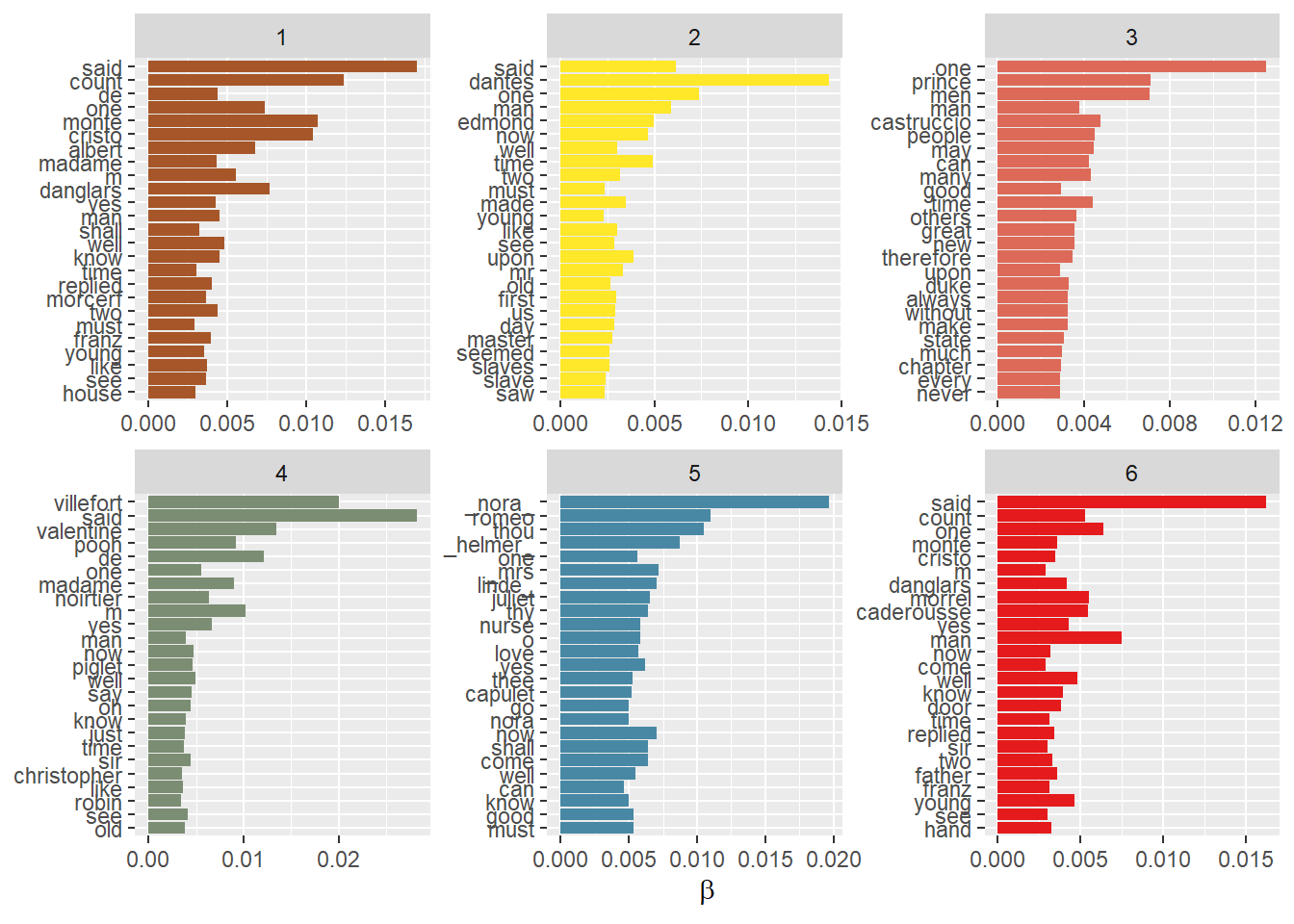
The Visualisation

Now that we have run the LDA model, we can visualize the results with a ggplot.

Check out my code

# Plot
broom::tidy(shuffle_lda, matrix = "beta") |>
  dplyr::group_by(topic) |>
  dplyr::slice_max(order_by = beta, n = 25) |>
  ggplot(aes(x= term |> reorder(beta), y= beta, fill=topic)) +
  geom_col() +
  coord_flip()+
  scale_fill_distiller(palette="Set1")+
  facet_wrap(~topic, scales = "free") +
  labs(x = NULL, y = expression(beta))+
  theme(legend.position = "none")

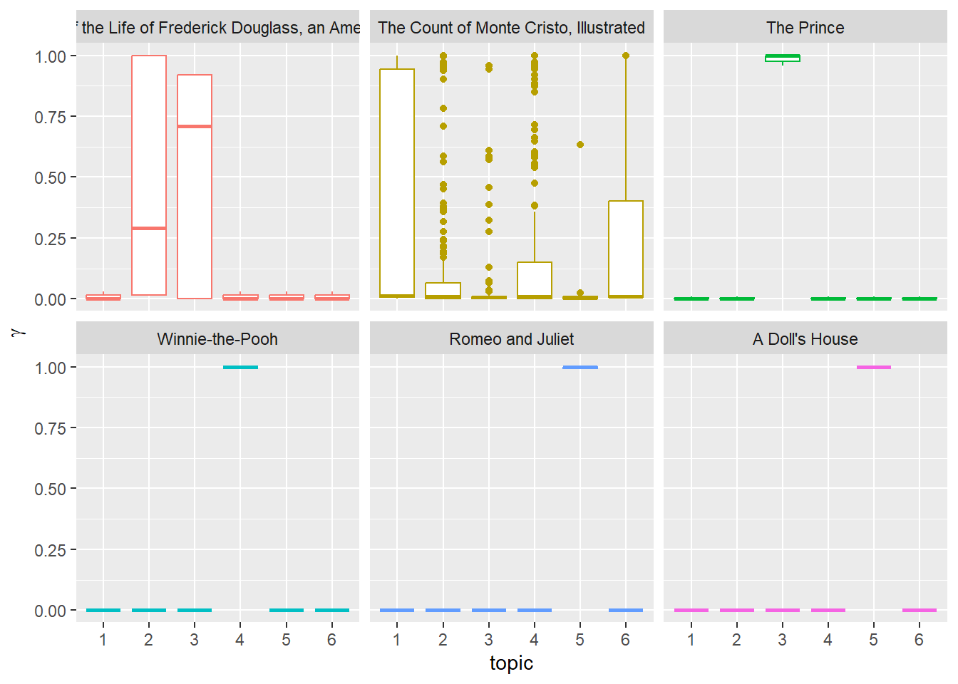
Second visual

The next image visualizes the relationships between each book and each topic. We can see that for some books (The Prince, Winnie-the-Pooh, Rome and Juliet, and A Doll’s House), there is a clear match (1 book, 1 topic), whereas the remaining two books (A Narrative of the Life of Frederick Douglass and the Count of Monte Cristo), the model was not able to match all chapters of the book to a single topic. The Dumas book, in particular, has its chapters spread out across all 6 topics. This may have something to do with book-length: the Count of Monte Cristo has far more chapters than any of the other books.

Check out my code

# Beta ####
words_beta <- broom::tidy(shuffle_lda, matrix = "beta") 

# Gamma ####
chapters_gamma <- broom::tidy(shuffle_lda, matrix = "gamma")

# Plot
broom::tidy(shuffle_lda, matrix = "gamma") |>
  tidyr::separate(document, c("title", "chapter"), sep = "_", convert = TRUE) |>
  dplyr::mutate(title = reorder(title, gamma * topic)) %>%
  ggplot(aes(factor(topic), gamma, color=title)) +
  geom_boxplot() +
  facet_wrap(~title) +
  labs(x = "topic", y = expression(gamma))+
  theme(legend.position = "none")

Heat Map

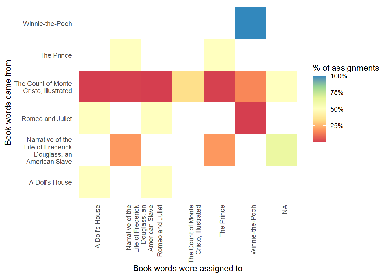
Finally, we use a heat map to visualize the success of the model. The only 100% success was Winnie-the-Pooh, for which all chapters were correctly assigned. The worst, again, was Count of Monte Cristo, with chapters assigned to every single one of the topics, and less than half of chapters assigned to the correct book.

Check out my code

# Save chapter classifications ####
chapter_classifications <- broom::tidy(shuffle_lda, matrix = "gamma") |>
  tidyr::separate(document, c("title", "chapter"), sep = "_", convert = TRUE)  %>%
  dplyr::group_by(title, chapter) %>%
  dplyr::slice_max(gamma) %>%
  dplyr::ungroup()

# Save most likely topics for each book ####
book_topics <- chapter_classifications %>%
  dplyr::count(title, topic) %>%
  dplyr::group_by(title) %>%
  dplyr::slice_max(n, n = 1) %>%
  dplyr::ungroup() %>%
  dplyr::transmute(consensus = title, topic)

# Join the results ####
chapter_classifications %>%
  dplyr::left_join(book_topics, by = "topic") %>%
  dplyr::filter(title != consensus)

# A tibble: 154 × 5
   title                                             chapter topic gamma conse…¹
   <chr>                                               <int> <int> <dbl> <chr>  
 1 A Doll's House                                          1     5 1.00  Romeo …
 2 A Doll's House                                          2     5 1.00  Romeo …
 3 A Doll's House                                          3     5 1.00  Romeo …
 4 Narrative of the Life of Frederick Douglass, an …       1     3 0.852 The Pr…
 5 Narrative of the Life of Frederick Douglass, an …       2     3 0.919 The Pr…
 6 Narrative of the Life of Frederick Douglass, an …       3     3 0.919 The Pr…
 7 Narrative of the Life of Frederick Douglass, an …       4     3 0.919 The Pr…
 8 Narrative of the Life of Frederick Douglass, an …       5     3 0.919 The Pr…
 9 Narrative of the Life of Frederick Douglass, an …       6     3 0.919 The Pr…
10 Narrative of the Life of Frederick Douglass, an …       7     3 0.919 The Pr…
# … with 144 more rows, and abbreviated variable name ¹consensus

Check out my code

# Add Document Term Matrix data to results and join book classifications ####
assignments <- broom::augment(shuffle_lda, data = shuffle_dtm) |>
  tidyr::separate(document, c("title", "chapter"), 
           sep = "_", convert = TRUE) %>%
  dplyr::left_join(book_topics, by = c(".topic" = "topic"), relationship="many-to-many")

# Visualise the result ####
assignments %>%
  dplyr::count(title, consensus, wt = count) %>%
  dplyr::mutate(across(c(title, consensus), ~str_wrap(., 20))) %>%
  dplyr::group_by(title) %>%
  dplyr::mutate(percent = n / sum(n)) %>%
  ggplot(aes(consensus, title, fill = percent)) +
  geom_tile() +
  scale_fill_distiller(palette = "Spectral", direction=1,label = percent_format()) +
  theme_minimal() +
  theme(axis.text.x = element_text(angle = 90, hjust = 1),
        panel.grid = element_blank()) +
  labs(x = "Book words were assigned to",
       y = "Book words came from",
       fill = "% of assignments")

--- title: "**Shufflebook**" title-block-banner: "#8596c7" subtitle: "*Shuffling is the only thing which Nature cannot undo.*<br>-- Arthur Eddington" date: "2023-02-21" categories: [literature,LDA,tidytext,books,gutenbergr] image: Monkey-typing.jpg description: "Using a Latent Dirichlet Allocation model to place shuffled book chapters back into their proper book." --- ## The Books The first step is downloading 6 books from Project Gutenberg. We are starting with 6 books with a wide range of topics and genres. ```{r packages} #| include: false library(gutenbergr) library(tidytext) library(tidyverse) ``` ```{r download} #| message=FALSE # Download books #### ## Books to break down #### shuffle_titles <- c( "Romeo and Juliet", "The Count of Monte Cristo, Illustrated", "A Doll's House", "Narrative of the Life of Frederick Douglass, an American Slave", "Winnie-the-Pooh", "The Prince" ) shuffle_books <- gutenberg_works(title %in% shuffle_titles) |> gutenberg_download(meta_fields = "title") ``` ## The Shuffling Now we break the books into chapters, and the chapters into words (using tidytext). ```{r include=FALSE} #| include: false library(tidytext) library(tidyverse) ``` ```{r shuffle} #| message=FALSE # Separate the books into chapters, and add an identifying column ("Chapter") concatenating the book title and chapter number break_chapters <- shuffle_books |> # Trim whitespace at beginning of text values dplyr::mutate(text = str_trim(text, side = "left")) |> # group by title dplyr::group_by(title) |> # mutate the chapter column to be the cumulative sum of the text column dplyr::mutate(chapter_number = cumsum(str_detect(text, regex("^chapter |^act ", ignore_case = TRUE)))) |> # ungroup the data dplyr::ungroup() |> # filter out the chapters that are not greater than 0 dplyr::filter(chapter_number > 0) |> # unite the title and chapter number columns into one column called chapter tidyr::unite(chapter, title, chapter_number) # Split into words chapter_word <- break_chapters |> # Unnest the tokens (words) in the text column tidytext::unnest_tokens(word, text) |> # Remove stopwords dplyr::anti_join(stopwords::stopwords("en", "snowball") |> as_tibble(), by=c("word"="value")) |> dplyr::count(chapter, word, sort = TRUE) ``` ## The (Attempted) Unshuffling Having split the books into words and removed all stopwords, we can now run an LDA model to estimate the probability that each word in a chapter belongs to a topic, and then use these word-topic associations to sort the chapters into their books. ```{r include=false} #| include: false library(tidytext) library(tidyverse) library(topicmodels) library(scales, warn.conflicts = FALSE) ``` ```{r LDA} #| message=FALSE # Create a document-term matrix from the chapter_word data frame shuffle_dtm <- chapter_word %>% tidytext::cast_dtm(chapter, word, n) # Estimate LDA shuffle_lda <- topicmodels::LDA(shuffle_dtm, # As many topics as books, but we can include more if we wanted to k = 6, # For reproduciblity control = list(seed = 1234)) ``` ## The Visualisation Now that we have run the LDA model, we can visualize the results with a ggplot. ```{r packages2} #| include: false library(tidytext, warn.conflicts = FALSE) library(tidyverse, warn.conflicts = FALSE) library(topicmodels, warn.conflicts = FALSE) library(scales, warn.conflicts = FALSE) ``` ```{r first visual} #| message=FALSE # Plot broom::tidy(shuffle_lda, matrix = "beta") |> dplyr::group_by(topic) |> dplyr::slice_max(order_by = beta, n = 25) |> ggplot(aes(x= term |> reorder(beta), y= beta, fill=topic)) + geom_col() + coord_flip()+ scale_fill_distiller(palette="Set1")+ facet_wrap(~topic, scales = "free") + labs(x = NULL, y = expression(beta))+ theme(legend.position = "none") ``` ## Second visual The next image visualizes the relationships between each book and each topic. We can see that for some books (The Prince, Winnie-the-Pooh, Rome and Juliet, and A Doll's House), there is a clear match (1 book, 1 topic), whereas the remaining two books (A Narrative of the Life of Frederick Douglass and the Count of Monte Cristo), the model was not able to match all chapters of the book to a single topic. The Dumas book, in particular, has its chapters spread out across all 6 topics. This may have something to do with book-length: the Count of Monte Cristo has far more chapters than any of the other books. ```{r packages3} #| include: false library(tidytext) library(tidyverse) library(topicmodels) library(scales, warn.conflicts = FALSE) ``` ```{r Visualising word-topic and book-topic relationships} #| message=FALSE # Beta #### words_beta <- broom::tidy(shuffle_lda, matrix = "beta") # Gamma #### chapters_gamma <- broom::tidy(shuffle_lda, matrix = "gamma") # Plot broom::tidy(shuffle_lda, matrix = "gamma") |> tidyr::separate(document, c("title", "chapter"), sep = "_", convert = TRUE) |> dplyr::mutate(title = reorder(title, gamma * topic)) %>% ggplot(aes(factor(topic), gamma, color=title)) + geom_boxplot() + facet_wrap(~title) + labs(x = "topic", y = expression(gamma))+ theme(legend.position = "none") ``` ## Heat Map Finally, we use a heat map to visualize the success of the model. The only 100% success was Winnie-the-Pooh, for which all chapters were correctly assigned. The worst, again, was Count of Monte Cristo, with chapters assigned to every single one of the topics, and less than half of chapters assigned to the correct book. ```{r packages4} #| include: false library(tidytext) library(tidyverse) library(topicmodels) library(scales) ``` ```{r tibble} #| message=FALSE # Save chapter classifications #### chapter_classifications <- broom::tidy(shuffle_lda, matrix = "gamma") |> tidyr::separate(document, c("title", "chapter"), sep = "_", convert = TRUE) %>% dplyr::group_by(title, chapter) %>% dplyr::slice_max(gamma) %>% dplyr::ungroup() # Save most likely topics for each book #### book_topics <- chapter_classifications %>% dplyr::count(title, topic) %>% dplyr::group_by(title) %>% dplyr::slice_max(n, n = 1) %>% dplyr::ungroup() %>% dplyr::transmute(consensus = title, topic) # Join the results #### chapter_classifications %>% dplyr::left_join(book_topics, by = "topic") %>% dplyr::filter(title != consensus) # Add Document Term Matrix data to results and join book classifications #### assignments <- broom::augment(shuffle_lda, data = shuffle_dtm) |> tidyr::separate(document, c("title", "chapter"), sep = "_", convert = TRUE) %>% dplyr::left_join(book_topics, by = c(".topic" = "topic"), relationship="many-to-many") # Visualise the result #### assignments %>% dplyr::count(title, consensus, wt = count) %>% dplyr::mutate(across(c(title, consensus), ~str_wrap(., 20))) %>% dplyr::group_by(title) %>% dplyr::mutate(percent = n / sum(n)) %>% ggplot(aes(consensus, title, fill = percent)) + geom_tile() + scale_fill_distiller(palette = "Spectral", direction=1,label = percent_format()) + theme_minimal() + theme(axis.text.x = element_text(angle = 90, hjust = 1), panel.grid = element_blank()) + labs(x = "Book words were assigned to", y = "Book words came from", fill = "% of assignments") ```