SpotifyStats

I hope the world sees the same person that you always were to me, and may all your favorite bands stay together
– Dawes

All Your Favorite Bands, 2015

In this session we use data from Spotify for Developers to analyze the musical characteristics of some of my favorite musicians.

Tokens

Here I save my tokens

Other prep work

First, I get an access token using my Spotify credentials. Then, I define a function for getting an artist’s Spotify ID based on their name.

Check out my code

library(tidyverse)
library(spotifyr, warn.conflicts = FALSE)

Sys.setenv(SPOTIFY_CLIENT_ID = my_spotify_id)

Sys.setenv(SPOTIFY_CLIENT_SECRET = my_spotify_secret)

#Access token ### 
spotify_access_token <- get_spotify_access_token()

#Define function for getting artist ID ###
spotify_id <- function(artist_name){

spotifyr::search_spotify(print(artist_name), type = "artist")|>
dplyr::select(id) |> 
dplyr::slice(1) |>
as.character()
}

Run main code

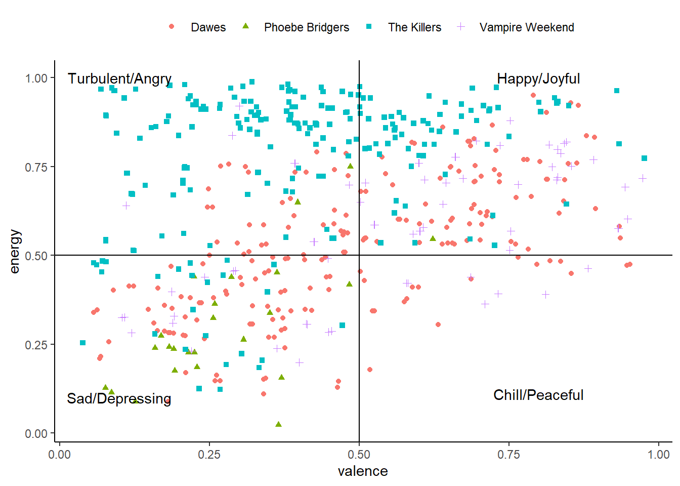
Now we can get the Spotify IDs for four of my favorite artists, create a data frame of their discographies, and conduct analyses on musical characteristics such as valence and energy.

Check out my code

#Get artist ID for Dawes, Phoebe Bridgers, Vampire Weekend, and The Killers ###
spotify_id("Dawes")

[1] "Dawes"

[1] "0CDUUM6KNRvgBFYIbWxJwV"

Check out my code

spotify_id("Phoebe Bridgers")

[1] "Phoebe Bridgers"

[1] "1r1uxoy19fzMxunt3ONAkG"

Check out my code

spotify_id("Vampire Weekend")

[1] "Vampire Weekend"

[1] "5BvJzeQpmsdsFp4HGUYUEx"

Check out my code

spotify_id("The Killers")

[1] "The Killers"

[1] "0C0XlULifJtAgn6ZNCW2eu"

Check out my code

#Make list of faves: Dawes, Phoebe Bridgers, Vampire Weekend, The Killers ###
favorites <- c("Dawes","Phoebe Bridgers","Vampire Weekend","The Killers")

#Create empty list
favorites_music <- list()

# for loop ##
for(i in favorites) {
  favorites_music[[i]] <- spotifyr::get_artist_audio_features(artist = print(i),
                                    include_groups = "album",
                                    authorization = spotify_access_token)
}

[1] "Dawes"
[1] "Phoebe Bridgers"
[1] "Vampire Weekend"
[1] "The Killers"

Check out my code

##Mood map of the 4 artists
favorites_music |>
  purrr::map_df(bind_rows)|>
  ggplot(aes(y=energy,x=valence,color=artist_name))+
  geom_point(aes(shape=artist_name))+
  geom_hline(yintercept = 0.5)+
  geom_vline(xintercept = 0.5)+
  annotate("text", x = 0.1, y = 1, label = "Turbulent/Angry")+
  annotate("text", x = 0.8, y = 1, label = "Happy/Joyful")+
  annotate("text", x = 0.1, y = 0.1, label = "Sad/Depressing")+
  annotate("text", x = 0.8, y = 0.11, label =     "Chill/Peaceful")+
  theme_classic()+
  theme(legend.position = "top",
        legend.title = element_blank())

The Valence Violin

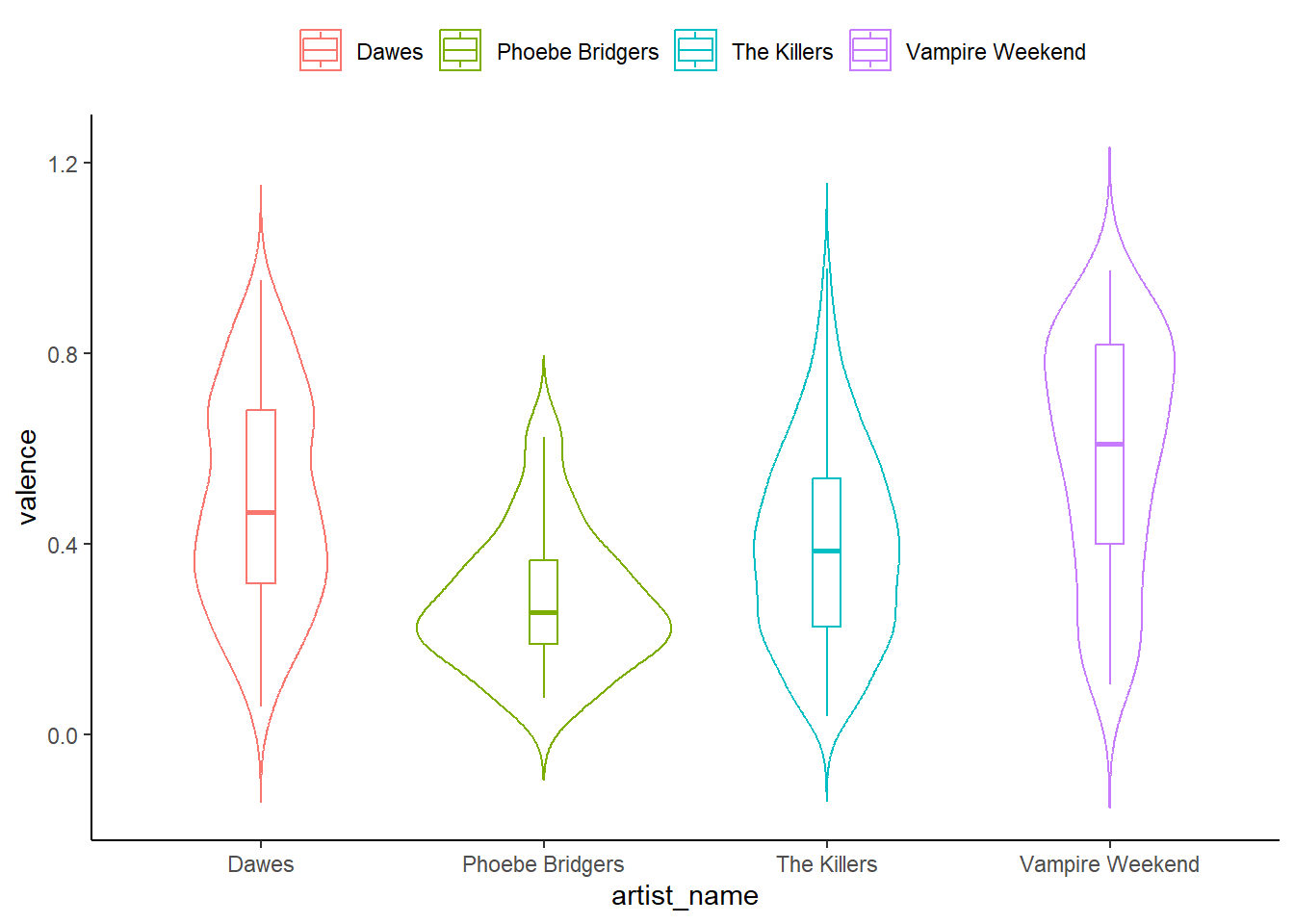
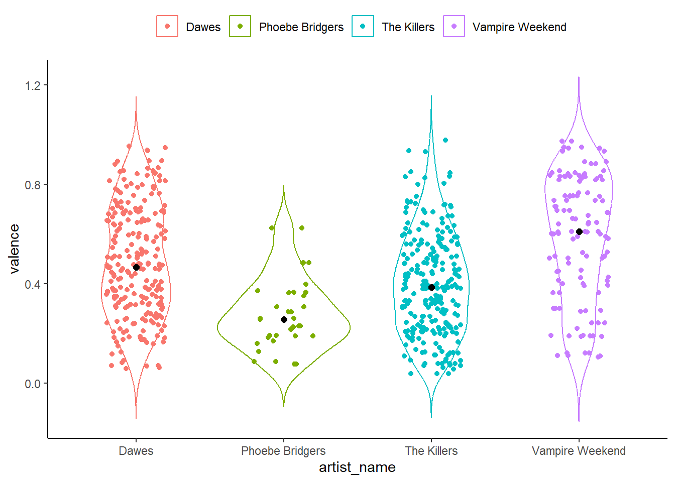
This final chart displays valence for each artist in the form of a violin plot. The plot is first shown with a boxplot overlaid, and then with the individual observations overlayed in a jitter formation (the median value is here shown in black).

Check out my code

##Violin chart of 4 artists
favorites_music |>
    purrr::map_df(bind_rows)|>
    ggplot(aes(x=artist_name,y=valence,color=artist_name))+
    geom_violin(trim=FALSE)+
    geom_boxplot(width=0.1)+
    theme_classic()+
    theme(legend.position = "top",
    legend.title = element_blank())

Check out my code

favorites_music |>
    purrr::map_df(bind_rows)|>
    ggplot(aes(x=artist_name,y=valence,color=artist_name))+
    geom_violin(trim=FALSE)+
    geom_jitter(shape=16, position=position_jitter(0.2))+
    stat_summary(fun=median, geom="point", size=2, color="black")+
    theme_classic()+
    theme(legend.position = "top",
    legend.title = element_blank())

We can see that Vampire Weekend has the longest range of valence values, as well as the highest median value. The music of Phoebe Bridgers, on the other hand, has a lower median and a tighter range.