Load data and build first, basic plot

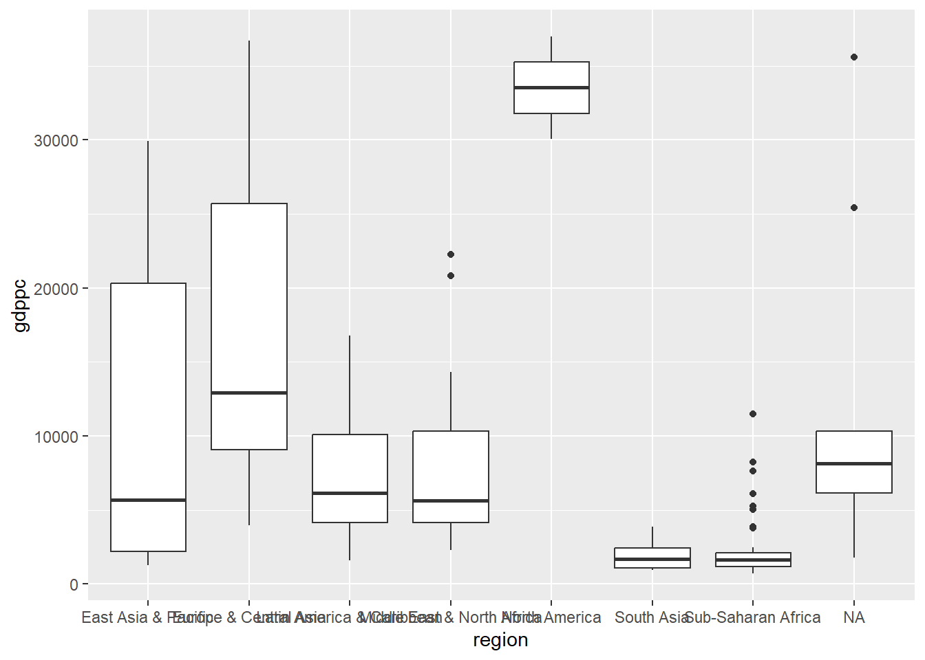
The data is pulled directly from Our World in Data’s GitHub repository using the read_csv function. Then, with just a few tweaks with the countrycode package, it’s ready to be fed into a box plot.

Check out my code

library(tidyverse)
library(countrycode)

# OWID repository for the Maddison Project data ####
owid_maddison_proj <- readr::read_csv("https://raw.githubusercontent.com/owid/owid-datasets/master/datasets/Maddison%20Project%20Database%202020%20(Bolt%20and%20van%20Zanden%20(2020))/Maddison%20Project%20Database%202020%20(Bolt%20and%20van%20Zanden%20(2020)).csv")

# Add regions and country codes ####
owid_maddison_proj_df <- owid_maddison_proj |>
  # rename variables 
  dplyr::rename(country=1,year=2,gdppc=3,pop=4,gdp=5) |>
  # Add country ISO code and region
  dplyr::mutate(iso3c = countrycode::countrycode(sourcevar = country, origin = "country.name", destination = "iso3c"),
                region = countrycode::countrycode(sourcevar = country, origin = "country.name", destination = "region"))

# A first visual ####
maddison_proj_1 <- owid_maddison_proj_df |>
  # Filter for 1990 ###
  dplyr::filter(year==1990) |>
  # Pipe into ggplot and define X and Y axis
  ggplot(aes(x=region,y=gdppc))+
  # Show a boxplot
  geom_boxplot()

# Let's send the result to the console to see it
maddison_proj_1

Reordering and Scaling

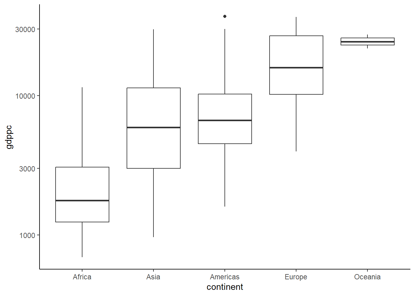
As a first step from an ugly duckling graph to a beautiful swan, we can use continents instead of regions and remove sub-regional aggregates. At the same time, we’ll add a variable to sort the continents in descending order of GDP per capita. This will look cleaner if we rescale the GDP per capita variable to a logarithmic scale (base 10). And to tie a nice bow on this new graph, we can use a theme to tidy up some colors and features.

Check out my code

library(tidyverse)
library(countrycode) 

# We save a new data frame with the continent option ####
owid_maddison_proj_df2 <- owid_maddison_proj_df |>
  # Add continent 
  dplyr::mutate(continent = countrycode::countrycode(sourcevar = iso3c, origin = "iso3c", destination = "continent"))

# New attempt ####
maddison_proj_2 <- owid_maddison_proj_df2 |>
  # Filter for the year we want ###
  dplyr::filter(year==1990, !is.na(continent)) |>
  # Group the data by continent
  dplyr::group_by(continent) |>
  # Create a new variable with the median of GDP per capita in each continent
  dplyr::mutate(m_gdppc = median(gdppc, na.rm=TRUE)) |>
  # Return to all data
  dplyr::ungroup() |>
  # Reorder the variable using factors
  dplyr::mutate(continent = fct_reorder(continent, m_gdppc)) |>
  # Pipe into ggplot and define X and Y axis
  ggplot(aes(x=continent,y=gdppc))+
  # Show a boxplot with outlier
  geom_boxplot()+
  # Scale log
  scale_y_log10()+
  # Clean theme with cleaner options
  theme_classic()+
  # We supress the legend everywhere with this option
  theme(legend.position = "none")

# See the result
maddison_proj_2

Time for a makeover

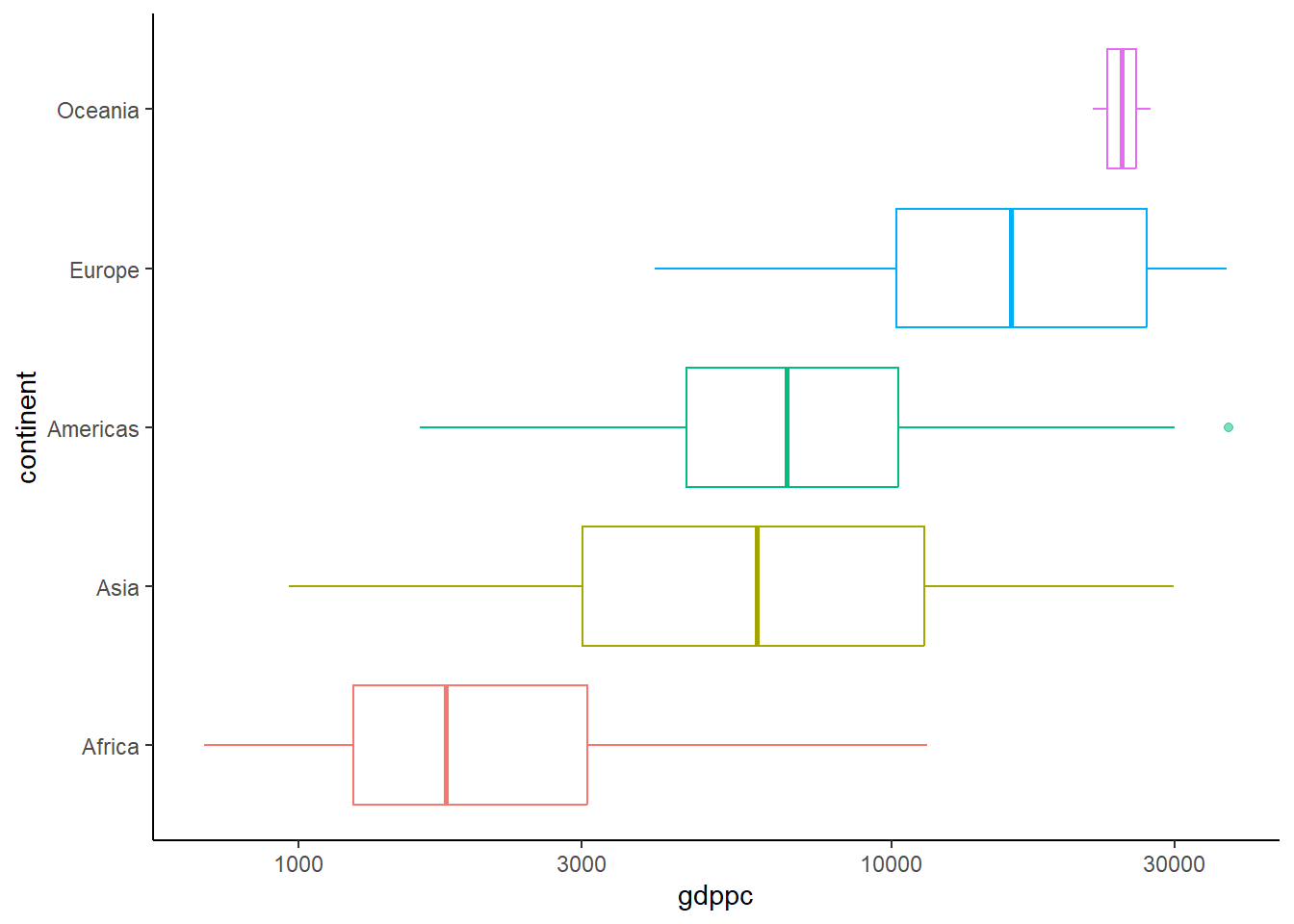
The data is now there in more or less the format we want to see it, but the graph isn’t very pretty. We can make it more readable and appealing by flipping the coordinates and adding some colors.

Check out my code

library(tidyverse)
library(RColorBrewer)

# A third visual ####
maddison_proj_3 <- owid_maddison_proj_df2 |>
  # Filter for the year we want ###
  dplyr::filter(year==1990, !is.na(continent)) |>
  # Group the data by continent
  dplyr::group_by(continent) |>
  # Create a new variable with the median of GDP per capita in each continent
  dplyr::mutate(m_gdppc = median(gdppc, na.rm=TRUE)) |>
  # Return to all data
  dplyr::ungroup() |>
  # Reorder the variable using factors
  dplyr::mutate(continent = fct_reorder(continent, m_gdppc)) |>
  # Pipe into ggplot and define X and Y axis
  ggplot(aes(x=continent,y=gdppc, color=continent))+
  # Show a boxplot
  geom_boxplot(outlier.alpha= 0.5)+
  # Scale log
  scale_y_log10()+
  # Flip X and Y coordinates
  coord_flip()+
  # Clean theme
  theme_classic()+
  theme(legend.position = "none")

maddison_proj_3

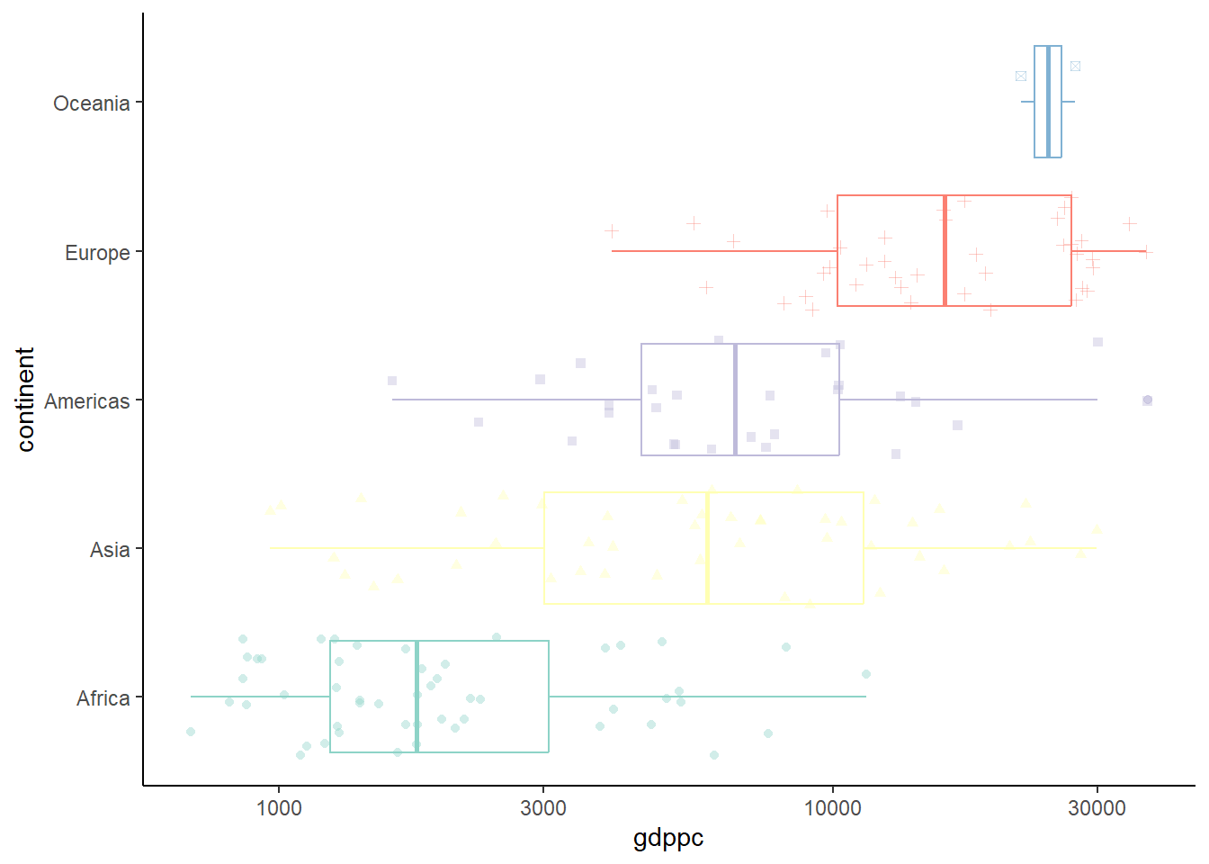
It would be nice to also see all the individual data points behind these boxes. Geom_jitter ensures that the dots don’t overlap. Using both different colors and different shapes for each continent is a fun aesthetic bonus.

Check out my code

library(tidyverse)
library(RColorBrewer)

# A fourth visual ####
maddison_proj_4 <- owid_maddison_proj_df2 |>
  # Filter for the year we want ###
  dplyr::filter(year==1990, !is.na(continent)) |>
  # Group the data by continent
  dplyr::group_by(continent) |>
  # Create a new variable with the median of GDP per capita in each continent
  dplyr::mutate(m_gdppc = median(gdppc, na.rm=TRUE)) |>
  # Return to all data
  dplyr::ungroup() |>
  # Reorder the variable using factors
  dplyr::mutate(continent = fct_reorder(continent, m_gdppc)) |>
  # Pipe into ggplot and define X and Y axis
  ggplot(aes(x=continent,y=gdppc, color=continent))+
  # Show a boxplot
  geom_boxplot(outlier.alpha= 0.5)+
  # Show jittered points colored by continent
  geom_jitter(aes(shape=continent), alpha=0.4)+
  # Scale log
  scale_y_log10()+
  # Color palette for continents
  scale_color_brewer(palette="Set3")+
  # Flip X and Y coordinates
  coord_flip()+
  # Clean theme
  theme_classic()+
  theme(legend.position = "none")

maddison_proj_4

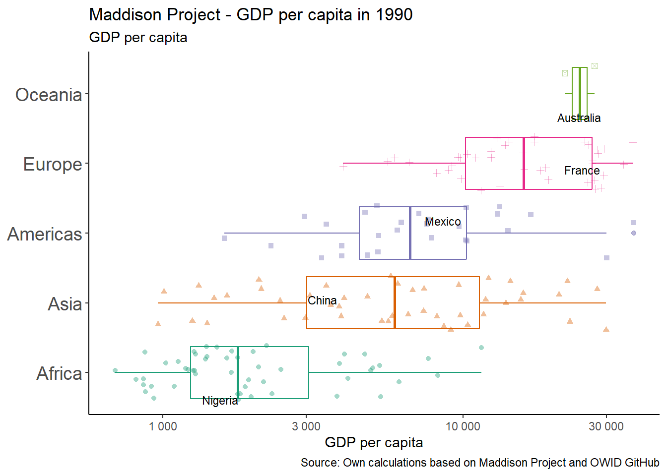
Put a label on it

Unlike your non-committal ex, we like labels. So let’s add some labels, titles and subtitles to the graph to make it crystal-clear. This includes a floating label for one example country in each continent.

Check out my code

library(tidyverse)
library(ggrepel)
library(RColorBrewer)

# A fifth visual ####
maddison_proj_5 <- owid_maddison_proj_df2 |>
  # Filter for the year we want ###
  dplyr::filter(year==1990, !is.na(continent)) |>
  # Group the data by continent
  dplyr::group_by(continent) |>
  # Create a new variable with the median of GDP per capita in each continent
  dplyr::mutate(m_gdppc = median(gdppc, na.rm=TRUE)) |>
  # Return to all data
  dplyr::ungroup() |>
  # Reorder the variable using factors
  dplyr::mutate(continent = fct_reorder(continent, m_gdppc)) |>
  # Pipe into ggplot and define X and Y axis
  ggplot(aes(x=continent,y=gdppc, color=continent))+
  # Show a boxplot
  geom_boxplot(outlier.alpha= 0.5)+
  # Show jittered points colored by continent
  geom_jitter(aes(shape=continent), alpha=0.4)+
  # Label Mexico, China, Nigeria
  geom_text_repel(data = . %>% 
                    dplyr::filter(country %in% c("Mexico","China","Nigeria","France","Australia"), year==1990),
                    aes(label=country), size=3, color="black", 
                    # Notice we add this to align the labels with the jittering
                    position = position_jitter(seed = 1))+
  # Scale log, breaks for a logged axis and space between thousands digits
  scale_y_continuous(trans = "log10",labels = scales::number_format(big.mark=" "))+
  # Color palette for continents
  scale_color_brewer(palette="Dark2")+
  # Flip X and Y coordinates
  coord_flip()+
  # Labels
  labs(x = NULL, y = "GDP per capita",
       title = "Maddison Project - GDP per capita in 1990",
       subtitle = "GDP per capita",
       caption = "Source: Own calculations based on Maddison Project and OWID GitHub") + 
  # Clean theme
  theme_classic()+
  # Increase size of continent axis label and drop the legend
  theme(legend.position = "none",
        axis.text.y = element_text(size = 14)
  )

maddison_proj_5

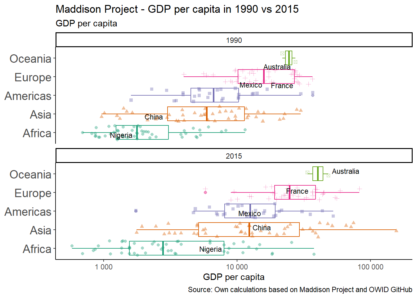
Fascinating faceting

Given that the Maddison Project has GDP per capita data for hundreds of years, it would be shame to look at only one point in time. So let’s start by comparing two years: 1990 and 2015. Facet_wrap is a beautiful way to show different parts of the same dataset with the same axes and structure.

Check out my code

library(tidyverse)
library(ggrepel)
library(RColorBrewer)

# A final visual ####
maddison_proj_6 <- owid_maddison_proj_df2 |>
  # Filter for the years we want ###
  dplyr::filter(year %in% c(1990,2015), !is.na(continent)) |>
  # Group the data by continent
  dplyr::group_by(year, continent) |>
  # Create a new variable with the median of GDP per capita in each continent
  dplyr::mutate(m_gdppc = median(gdppc, na.rm=TRUE)) |>
  # Return to all data
  dplyr::ungroup() |>
  # Reorder the variable using factors
  dplyr::mutate(continent = fct_reorder(continent, m_gdppc)) |>
  # Pipe into ggplot and define X and Y axis
  ggplot(aes(x=continent,y=gdppc, color=continent))+
  # Show a boxplot
  geom_boxplot(outlier.alpha= 0.5)+
  # Show jittered points colored by continent
  geom_jitter(aes(shape=continent), alpha=0.4)+
  # Label Mexico, China, Nigeria
  geom_text_repel(data = . %>% 
                    dplyr::filter(country %in% c("Mexico","China","Nigeria","France","Australia")),
                    aes(label=country), size=3, color="black", 
                    # Notice we add this to align the labels with the jittering
                    position = position_jitter(seed = 1))+
  # Scale log, breaks for a logged axis and space between thousands digits
  scale_y_continuous(trans = "log10",labels = scales::number_format(big.mark=" "))+
  # Color palette for continents
  scale_color_brewer(palette="Dark2")+
  # Flip X and Y coordinates
  coord_flip()+
  # Faceting
  facet_wrap(~year, nrow=2)+
  # Labels
  labs(x = NULL, y = "GDP per capita",
       title = "Maddison Project - GDP per capita in 1990 vs 2015",
       subtitle = "GDP per capita",
       caption = "Source: Own calculations based on Maddison Project and OWID GitHub") + 
  # Clean theme
  theme_classic()+
  # Increase size of continent axis label and drop the legend
  theme(legend.position = "none",
        axis.text.y = element_text(size = 14)
  )

maddison_proj_6

And just like that, our ugly duckling is a swan…our nerdy protagonist has taken off her glasses and become a princess.

Ggiraph-iti 🦒🖌

As lovely as the last graph was, there’s still one thing that would really take it over the top. As someone who has frequently been glared and/or yelled at in museums for wanting to touch the art, I know that human nature is never content to simply observe – we want to interact. So let’s give the people what they want and make this chart interactive, using a handy little package called ggiraph.

Check out my code

library(tidyverse)
library(RColorBrewer)
library(ggiraph)    # To create interactive plots
library(patchwork)  # To sew 'em together

# Set default css properties for girafe 
css_default_hover <- girafe_css_bicolor(primary = "cyan", secondary = "pink")

set_girafe_defaults(
  opts_hover = opts_hover(css = css_default_hover),
  opts_zoom = opts_zoom(min = 1, max = 4),
  opts_tooltip = opts_tooltip(css = "padding:3px;background-color:#333333;color:white;"),
  opts_sizing = opts_sizing(rescale = TRUE),
  opts_toolbar = opts_toolbar(saveaspng = FALSE, position = "bottom", delay_mouseout = 5000)
)


# GDP per capita through time by continent ####
maddison_time <- owid_maddison_proj_df2 |>
  dplyr::filter(year>=1950,!is.na(continent)) |>
  # Create summary statistics by year and continent
  dplyr::group_by(year, continent) |>
  dplyr::summarise(m_gdppc = median(gdppc, na.rm=TRUE)) |>
  # Feed to ggplot
  ggplot(aes(x=year,y=m_gdppc, color=continent))+
  # Notice the _interactive and the content in the aesthetics
  geom_path_interactive(aes(data_id=continent, tooltip=continent))+
  scale_y_log10()+
  scale_color_brewer(palette="Set3")+
  labs(x = NULL, y = "GDP per capita") + 
  theme_classic()+
  theme(legend.position = "none")

# Distribution of GDP per capita by continent  ####
maddison_continent <- owid_maddison_proj_df2 |>
  dplyr::filter(year>=1950,!is.na(continent)) |>
  ggplot(aes(x=continent,y=gdppc, color=continent, fill=continent))+
  # Add points and a violin background
  geom_jitter(color="grey90")+
  geom_violin(alpha=0.4)+
  # Add interactive box plot, with same parameters as the interactive geom_path above
  geom_boxplot_interactive(aes(data_id=continent, tooltip=continent))+
  scale_y_log10()+
  scale_fill_brewer(palette="Set3")+
  coord_flip()+
  labs(x = NULL, y = "GDP per capita") + 
  theme_classic()+
  theme(legend.position = "none")

# Combine the two plots into one ####
ggiraph::girafe(
  # With patchwork we can just add the plots together to appear side by side
  ggobj = maddison_time + maddison_continent +
    # Here we add annotations
    plot_annotation(
  title = 'Maddison Project - GDP per capita since 1950',
  subtitle = 'GDP per capita by continent',
  caption = 'Source: Own calculations based on Maddison Project and OWID'
),
  width_svg = 10,
  height_svg = 6
)

--- title: "**How to give a chart a makeover 📊💄**" title-block-banner: "#8596c7" subtitle: "*A picture may be worth a thousand words, but a formula is worth a thousand pictures.*<br>-- Edsger Dijkstra" date: "2023-04-13" image: makeover.gif categories: [ggplot2,plotly,ggiraph,countrycode,interactive] description: "Using data from the Maddison Project to practice the art of finetuning graphs." --- # Load data and build first, basic plot The data is pulled directly from Our World in Data's GitHub repository using the read_csv function. Then, with just a few tweaks with the countrycode package, it's ready to be fed into a box plot. ```{r load-data-first-plot} library(tidyverse) library(countrycode) # OWID repository for the Maddison Project data #### owid_maddison_proj <- readr::read_csv("https://raw.githubusercontent.com/owid/owid-datasets/master/datasets/Maddison%20Project%20Database%202020%20(Bolt%20and%20van%20Zanden%20(2020))/Maddison%20Project%20Database%202020%20(Bolt%20and%20van%20Zanden%20(2020)).csv") # Add regions and country codes #### owid_maddison_proj_df <- owid_maddison_proj |> # rename variables dplyr::rename(country=1,year=2,gdppc=3,pop=4,gdp=5) |> # Add country ISO code and region dplyr::mutate(iso3c = countrycode::countrycode(sourcevar = country, origin = "country.name", destination = "iso3c"), region = countrycode::countrycode(sourcevar = country, origin = "country.name", destination = "region")) # A first visual #### maddison_proj_1 <- owid_maddison_proj_df |> # Filter for 1990 ### dplyr::filter(year==1990) |> # Pipe into ggplot and define X and Y axis ggplot(aes(x=region,y=gdppc))+ # Show a boxplot geom_boxplot() # Let's send the result to the console to see it maddison_proj_1 ``` # Reordering and Scaling As a first step from an ugly duckling graph to a beautiful swan, we can use continents instead of regions and remove sub-regional aggregates. At the same time, we'll add a variable to sort the continents in descending order of GDP per capita. This will look cleaner if we rescale the GDP per capita variable to a logarithmic scale (base 10). And to tie a nice bow on this new graph, we can use a theme to tidy up some colors and features. ```{r second-graph} library(tidyverse) library(countrycode) # We save a new data frame with the continent option #### owid_maddison_proj_df2 <- owid_maddison_proj_df |> # Add continent dplyr::mutate(continent = countrycode::countrycode(sourcevar = iso3c, origin = "iso3c", destination = "continent")) # New attempt #### maddison_proj_2 <- owid_maddison_proj_df2 |> # Filter for the year we want ### dplyr::filter(year==1990, !is.na(continent)) |> # Group the data by continent dplyr::group_by(continent) |> # Create a new variable with the median of GDP per capita in each continent dplyr::mutate(m_gdppc = median(gdppc, na.rm=TRUE)) |> # Return to all data dplyr::ungroup() |> # Reorder the variable using factors dplyr::mutate(continent = fct_reorder(continent, m_gdppc)) |> # Pipe into ggplot and define X and Y axis ggplot(aes(x=continent,y=gdppc))+ # Show a boxplot with outlier geom_boxplot()+ # Scale log scale_y_log10()+ # Clean theme with cleaner options theme_classic()+ # We supress the legend everywhere with this option theme(legend.position = "none") # See the result maddison_proj_2 ``` # Time for a makeover The data is now there in more or less the format we want to see it, but the graph isn't very pretty. We can make it more readable and appealing by flipping the coordinates and adding some colors. ```{r graph-numero-3} library(tidyverse) library(RColorBrewer) # A third visual #### maddison_proj_3 <- owid_maddison_proj_df2 |> # Filter for the year we want ### dplyr::filter(year==1990, !is.na(continent)) |> # Group the data by continent dplyr::group_by(continent) |> # Create a new variable with the median of GDP per capita in each continent dplyr::mutate(m_gdppc = median(gdppc, na.rm=TRUE)) |> # Return to all data dplyr::ungroup() |> # Reorder the variable using factors dplyr::mutate(continent = fct_reorder(continent, m_gdppc)) |> # Pipe into ggplot and define X and Y axis ggplot(aes(x=continent,y=gdppc, color=continent))+ # Show a boxplot geom_boxplot(outlier.alpha= 0.5)+ # Scale log scale_y_log10()+ # Flip X and Y coordinates coord_flip()+ # Clean theme theme_classic()+ theme(legend.position = "none") maddison_proj_3 ``` It would be nice to also see all the individual data points behind these boxes. Geom_jitter ensures that the dots don't overlap. Using both different colors and different shapes for each continent is a fun aesthetic bonus. ```{r jitter} library(tidyverse) library(RColorBrewer) # A fourth visual #### maddison_proj_4 <- owid_maddison_proj_df2 |> # Filter for the year we want ### dplyr::filter(year==1990, !is.na(continent)) |> # Group the data by continent dplyr::group_by(continent) |> # Create a new variable with the median of GDP per capita in each continent dplyr::mutate(m_gdppc = median(gdppc, na.rm=TRUE)) |> # Return to all data dplyr::ungroup() |> # Reorder the variable using factors dplyr::mutate(continent = fct_reorder(continent, m_gdppc)) |> # Pipe into ggplot and define X and Y axis ggplot(aes(x=continent,y=gdppc, color=continent))+ # Show a boxplot geom_boxplot(outlier.alpha= 0.5)+ # Show jittered points colored by continent geom_jitter(aes(shape=continent), alpha=0.4)+ # Scale log scale_y_log10()+ # Color palette for continents scale_color_brewer(palette="Set3")+ # Flip X and Y coordinates coord_flip()+ # Clean theme theme_classic()+ theme(legend.position = "none") maddison_proj_4 ``` # Put a label on it Unlike your non-committal ex, we like labels. So let's add some labels, titles and subtitles to the graph to make it crystal-clear. This includes a floating label for one example country in each continent. ```{r labeling} library(tidyverse) library(ggrepel) library(RColorBrewer) # A fifth visual #### maddison_proj_5 <- owid_maddison_proj_df2 |> # Filter for the year we want ### dplyr::filter(year==1990, !is.na(continent)) |> # Group the data by continent dplyr::group_by(continent) |> # Create a new variable with the median of GDP per capita in each continent dplyr::mutate(m_gdppc = median(gdppc, na.rm=TRUE)) |> # Return to all data dplyr::ungroup() |> # Reorder the variable using factors dplyr::mutate(continent = fct_reorder(continent, m_gdppc)) |> # Pipe into ggplot and define X and Y axis ggplot(aes(x=continent,y=gdppc, color=continent))+ # Show a boxplot geom_boxplot(outlier.alpha= 0.5)+ # Show jittered points colored by continent geom_jitter(aes(shape=continent), alpha=0.4)+ # Label Mexico, China, Nigeria geom_text_repel(data = . %>% dplyr::filter(country %in% c("Mexico","China","Nigeria","France","Australia"), year==1990), aes(label=country), size=3, color="black", # Notice we add this to align the labels with the jittering position = position_jitter(seed = 1))+ # Scale log, breaks for a logged axis and space between thousands digits scale_y_continuous(trans = "log10",labels = scales::number_format(big.mark=" "))+ # Color palette for continents scale_color_brewer(palette="Dark2")+ # Flip X and Y coordinates coord_flip()+ # Labels labs(x = NULL, y = "GDP per capita", title = "Maddison Project - GDP per capita in 1990", subtitle = "GDP per capita", caption = "Source: Own calculations based on Maddison Project and OWID GitHub") + # Clean theme theme_classic()+ # Increase size of continent axis label and drop the legend theme(legend.position = "none", axis.text.y = element_text(size = 14) ) maddison_proj_5 ``` # Fascinating faceting Given that the Maddison Project has GDP per capita data for hundreds of years, it would be shame to look at only one point in time. So let's start by comparing two years: 1990 and 2015. Facet_wrap is a beautiful way to show different parts of the same dataset with the same axes and structure. ```{r facets} library(tidyverse) library(ggrepel) library(RColorBrewer) # A final visual #### maddison_proj_6 <- owid_maddison_proj_df2 |> # Filter for the years we want ### dplyr::filter(year %in% c(1990,2015), !is.na(continent)) |> # Group the data by continent dplyr::group_by(year, continent) |> # Create a new variable with the median of GDP per capita in each continent dplyr::mutate(m_gdppc = median(gdppc, na.rm=TRUE)) |> # Return to all data dplyr::ungroup() |> # Reorder the variable using factors dplyr::mutate(continent = fct_reorder(continent, m_gdppc)) |> # Pipe into ggplot and define X and Y axis ggplot(aes(x=continent,y=gdppc, color=continent))+ # Show a boxplot geom_boxplot(outlier.alpha= 0.5)+ # Show jittered points colored by continent geom_jitter(aes(shape=continent), alpha=0.4)+ # Label Mexico, China, Nigeria geom_text_repel(data = . %>% dplyr::filter(country %in% c("Mexico","China","Nigeria","France","Australia")), aes(label=country), size=3, color="black", # Notice we add this to align the labels with the jittering position = position_jitter(seed = 1))+ # Scale log, breaks for a logged axis and space between thousands digits scale_y_continuous(trans = "log10",labels = scales::number_format(big.mark=" "))+ # Color palette for continents scale_color_brewer(palette="Dark2")+ # Flip X and Y coordinates coord_flip()+ # Faceting facet_wrap(~year, nrow=2)+ # Labels labs(x = NULL, y = "GDP per capita", title = "Maddison Project - GDP per capita in 1990 vs 2015", subtitle = "GDP per capita", caption = "Source: Own calculations based on Maddison Project and OWID GitHub") + # Clean theme theme_classic()+ # Increase size of continent axis label and drop the legend theme(legend.position = "none", axis.text.y = element_text(size = 14) ) maddison_proj_6 ``` And just like that, our ugly duckling is a swan...our nerdy protagonist has taken off her glasses and become a princess. # Ggiraph-iti 🦒🖌 As lovely as the last graph was, there's still one thing that would really take it over the top. As someone who has frequently been glared and/or yelled at in museums for wanting to touch the art, I know that human nature is never content to simply observe -- we want to interact. So let's give the people what they want and make this chart interactive, using a handy little package called ggiraph. ```{r interactivity} library(tidyverse) library(RColorBrewer) library(ggiraph) # To create interactive plots library(patchwork) # To sew 'em together # Set default css properties for girafe css_default_hover <- girafe_css_bicolor(primary = "cyan", secondary = "pink") set_girafe_defaults( opts_hover = opts_hover(css = css_default_hover), opts_zoom = opts_zoom(min = 1, max = 4), opts_tooltip = opts_tooltip(css = "padding:3px;background-color:#333333;color:white;"), opts_sizing = opts_sizing(rescale = TRUE), opts_toolbar = opts_toolbar(saveaspng = FALSE, position = "bottom", delay_mouseout = 5000) ) # GDP per capita through time by continent #### maddison_time <- owid_maddison_proj_df2 |> dplyr::filter(year>=1950,!is.na(continent)) |> # Create summary statistics by year and continent dplyr::group_by(year, continent) |> dplyr::summarise(m_gdppc = median(gdppc, na.rm=TRUE)) |> # Feed to ggplot ggplot(aes(x=year,y=m_gdppc, color=continent))+ # Notice the _interactive and the content in the aesthetics geom_path_interactive(aes(data_id=continent, tooltip=continent))+ scale_y_log10()+ scale_color_brewer(palette="Set3")+ labs(x = NULL, y = "GDP per capita") + theme_classic()+ theme(legend.position = "none") # Distribution of GDP per capita by continent #### maddison_continent <- owid_maddison_proj_df2 |> dplyr::filter(year>=1950,!is.na(continent)) |> ggplot(aes(x=continent,y=gdppc, color=continent, fill=continent))+ # Add points and a violin background geom_jitter(color="grey90")+ geom_violin(alpha=0.4)+ # Add interactive box plot, with same parameters as the interactive geom_path above geom_boxplot_interactive(aes(data_id=continent, tooltip=continent))+ scale_y_log10()+ scale_fill_brewer(palette="Set3")+ coord_flip()+ labs(x = NULL, y = "GDP per capita") + theme_classic()+ theme(legend.position = "none") # Combine the two plots into one #### ggiraph::girafe( # With patchwork we can just add the plots together to appear side by side ggobj = maddison_time + maddison_continent + # Here we add annotations plot_annotation( title = 'Maddison Project - GDP per capita since 1950', subtitle = 'GDP per capita by continent', caption = 'Source: Own calculations based on Maddison Project and OWID' ), width_svg = 10, height_svg = 6 ) ```